Как найти обратную функцию для гиперболы - AutoPluse.ru

From Wikipedia, the free encyclopedia

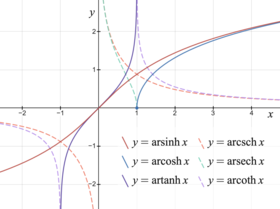
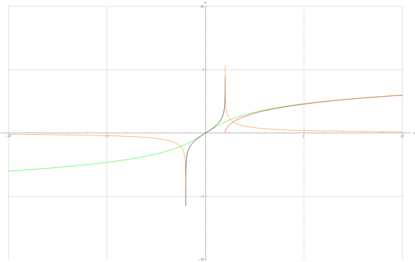
Graphs of the inverse hyperbolic functions

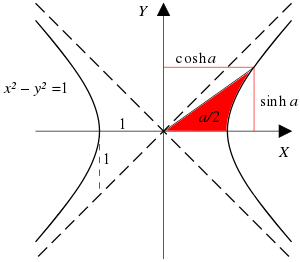
The hyperbolic functions sinh, cosh, and tanh with respect to a unit hyperbola are analogous to circular functions sin, cos, tan with respect to a unit circle. The argument to the hyperbolic functions is a hyperbolic angle measure.

In mathematics, the inverse hyperbolic functions are inverses of the hyperbolic functions, analogous to the inverse circular functions. There are six in common use: inverse hyperbolic sine, inverse hyperbolic cosine, inverse hyperbolic tangent, inverse hyperbolic cosecant, inverse hyperbolic secant, and inverse hyperbolic cotangent. They are commonly denoted by the symbols for the hyperbolic functions, prefixed with arc- or ar-.

For a given value of a hyperbolic function, the inverse hyperbolic function provides the corresponding hyperbolic angle measure, for example and Hyperbolic angle measure is the length of an arc of a unit hyperbola $x^{2}-y^{2}=1$ as measured in the Lorentzian plane (not the length of a hyperbolic arc in the Euclidean plane), and twice the area of the corresponding hyperbolic sector. This is analogous to the way circular angle measure is the arc length of an arc of the unit circle in the Euclidean plane or twice the area of the corresponding circular sector. Alternately hyperbolic angle is the area of a sector of the hyperbola Some authors call the inverse hyperbolic functions hyperbolic area functions.^[1]

Hyperbolic functions occur in the calculations of angles and distances in hyperbolic geometry. It also occurs in the solutions of many linear differential equations (such as the equation defining a catenary), cubic equations, and Laplace’s equation in Cartesian coordinates. Laplace’s equations are important in many areas of physics, including electromagnetic theory, heat transfer, fluid dynamics, and special relativity.

Notation[edit]

A ray through the unit hyperbola ${displaystyle x^{2} - y^{2} = 1}$ in the point , where is twice the area between the ray, the hyperbola, and the -axis

The earliest and most widely adopted symbols use the prefix arc- (that is: arcsinh, arccosh, arctanh, arcsech, arccsch, arccoth), by analogy with the inverse circular functions (arcsin, etc.). For a unit hyperbola («Lorentzian circle») in the Lorentzian plane (pseudo-Euclidean plane of signature (1, 1))^[2] or in the hyperbolic number plane,^[3] the hyperbolic angle measure (argument to the hyperbolic functions) is indeed the arc length of a hyperbolic arc.

Also common is the notation ${displaystyle sinh ^{-1},}$ ${displaystyle cosh ^{-1},}$ etc.,^[4]^[5] although care must be taken to avoid misinterpretations of the superscript −1 as an exponent. The standard convention is that ${displaystyle sinh ^{-1}x}$ or ${displaystyle sinh ^{-1}(x)}$ means the inverse function while ${displaystyle (sinh x)^{-1}}$ or ${displaystyle sinh(x)^{-1}}$ means the reciprocal Especially inconsistent is the conventional use of positive integer superscripts to indicate an exponent rather than function composition, e.g. ${displaystyle sinh ^{2}x}$ conventionally means ${displaystyle (sinh x)^{2}}$ and not

Because the argument of hyperbolic functions is not the arclength of a hyperbolic arc in the Euclidean plane, some authors have condemned the prefix arc-, arguing that the prefix ar- (for area) or arg- (for argument) should be preferred.^[6] Following this recommendation, the ISO 80000-2 standard abbreviations use the prefix ar- (that is: arsinh, arcosh, artanh, arsech, arcsch, arcoth).

In computer programming languages, inverse circular and hyperbolic functions are often named with the shorter prefix a- (asinh, etc.).

This article will consistently adopt the prefix ar- for convenience.

Definitions in terms of logarithms[edit]

Since the hyperbolic functions are quadratic rational functions of the exponential function they may be solved using the quadratic formula and then written in terms of the natural logarithm.

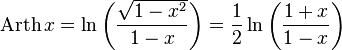
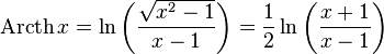
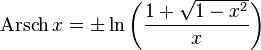
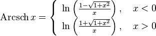
${displaystyle {begin{aligned}operatorname {arsinh} x&=ln left(x+{sqrt {x^{2}+1}}right)&-infty &<x<infty ,\[10mu]operatorname {arcosh} x&=ln left(x+{sqrt {x^{2}-1}}right)&1&leq x<infty ,\[10mu]operatorname {artanh} x&={frac {1}{2}}ln {frac {1+x}{1-x}}&-1&<x<1,\[10mu]operatorname {arcsch} x&=ln left({frac {1}{x}}+{sqrt {{frac {1}{x^{2}}}+1}}right)&-infty &<x<infty , xneq 0,\[10mu]operatorname {arsech} x&=ln left({frac {1}{x}}+{sqrt {{frac {1}{x^{2}}}-1}}right)&0&<xleq 1,\[10mu]operatorname {arcoth} x&={frac {1}{2}}ln {frac {x+1}{x-1}}&-infty &<x<-1 {text{or}} 1<x<infty .end{aligned}}}$

For complex arguments, the inverse circular and hyperbolic functions, the square root, and the natural logarithm are all multi-valued functions.

Addition formulae[edit]

${displaystyle operatorname {arsinh} upm operatorname {arsinh} v=operatorname {arsinh} left(u{sqrt {1+v^{2}}}pm v{sqrt {1+u^{2}}}right)}$

${displaystyle operatorname {arcosh} upm operatorname {arcosh} v=operatorname {arcosh} left(uvpm {sqrt {(u^{2}-1)(v^{2}-1)}}right)}$

${displaystyle operatorname {artanh} upm operatorname {artanh} v=operatorname {artanh} left({frac {upm v}{1pm uv}}right)}$

${displaystyle operatorname {arcoth} upm operatorname {arcoth} v=operatorname {arcoth} left({frac {1pm uv}{upm v}}right)}$

${displaystyle {begin{aligned}operatorname {arsinh} u+operatorname {arcosh} v&=operatorname {arsinh} left(uv+{sqrt {(1+u^{2})(v^{2}-1)}}right)\&=operatorname {arcosh} left(v{sqrt {1+u^{2}}}+u{sqrt {v^{2}-1}}right)end{aligned}}}$

Other identities[edit]

${displaystyle {begin{aligned}2operatorname {arcosh} x&=operatorname {arcosh} (2x^{2}-1)&quad {hbox{ for }}xgeq 1\4operatorname {arcosh} x&=operatorname {arcosh} (8x^{4}-8x^{2}+1)&quad {hbox{ for }}xgeq 1\2operatorname {arsinh} x&=operatorname {arcosh} (2x^{2}+1)&quad {hbox{ for }}xgeq 0\4operatorname {arsinh} x&=operatorname {arcosh} (8x^{4}+8x^{2}+1)&quad {hbox{ for }}xgeq 0end{aligned}}}$

${displaystyle ln(x)=operatorname {arcosh} left({frac {x^{2}+1}{2x}}right)=operatorname {arsinh} left({frac {x^{2}-1}{2x}}right)=operatorname {artanh} left({frac {x^{2}-1}{x^{2}+1}}right)}$

Composition of hyperbolic and inverse hyperbolic functions[edit]

${displaystyle {begin{aligned}&sinh(operatorname {arcosh} x)={sqrt {x^{2}-1}}quad {text{for}}quad |x|>1\&sinh(operatorname {artanh} x)={frac {x}{sqrt {1-x^{2}}}}quad {text{for}}quad -1<x<1\&cosh(operatorname {arsinh} x)={sqrt {1+x^{2}}}\&cosh(operatorname {artanh} x)={frac {1}{sqrt {1-x^{2}}}}quad {text{for}}quad -1<x<1\&tanh(operatorname {arsinh} x)={frac {x}{sqrt {1+x^{2}}}}\&tanh(operatorname {arcosh} x)={frac {sqrt {x^{2}-1}}{x}}quad {text{for}}quad |x|>1end{aligned}}}$

Composition of inverse hyperbolic and circular functions[edit]

${displaystyle operatorname {arsinh} left(tan alpha right)=operatorname {artanh} left(sin alpha right)=ln left({frac {1+sin alpha }{cos alpha }}right)=pm operatorname {arcosh} left({frac {1}{cos alpha }}right)}$

{displaystyle ln left(left|tan alpha right|right)=-operatorname {artanh} left(cos 2alpha right)}

^[7]

Conversions[edit]

${displaystyle ln x=operatorname {artanh} left({frac {x^{2}-1}{x^{2}+1}}right)=operatorname {arsinh} left({frac {x^{2}-1}{2x}}right)=pm operatorname {arcosh} left({frac {x^{2}+1}{2x}}right)}$

${displaystyle operatorname {artanh} x=operatorname {arsinh} left({frac {x}{sqrt {1-x^{2}}}}right)=pm operatorname {arcosh} left({frac {1}{sqrt {1-x^{2}}}}right)}$

${displaystyle operatorname {arsinh} x=operatorname {artanh} left({frac {x}{sqrt {1+x^{2}}}}right)=pm operatorname {arcosh} left({sqrt {1+x^{2}}}right)}$

${displaystyle operatorname {arcosh} x=left|operatorname {arsinh} left({sqrt {x^{2}-1}}right)right|=left|operatorname {artanh} left({frac {sqrt {x^{2}-1}}{x}}right)right|}$

Derivatives[edit]

${displaystyle {begin{aligned}{frac {d}{dx}}operatorname {arsinh} x&{}={frac {1}{sqrt {x^{2}+1}}},{text{ for all real }}x\{frac {d}{dx}}operatorname {arcosh} x&{}={frac {1}{sqrt {x^{2}-1}}},{text{ for all real }}x>1\{frac {d}{dx}}operatorname {artanh} x&{}={frac {1}{1-x^{2}}},{text{ for all real }}|x|<1\{frac {d}{dx}}operatorname {arcoth} x&{}={frac {1}{1-x^{2}}},{text{ for all real }}|x|>1\{frac {d}{dx}}operatorname {arsech} x&{}={frac {-1}{x{sqrt {1-x^{2}}}}},{text{ for all real }}xin (0,1)\{frac {d}{dx}}operatorname {arcsch} x&{}={frac {-1}{|x|{sqrt {1+x^{2}}}}},{text{ for all real }}x{text{, except }}0\end{aligned}}}$

For an example differentiation: let θ = arsinh x, so (where sinh² θ = (sinh θ)²):

${displaystyle {frac {d,operatorname {arsinh} x}{dx}}={frac {dtheta }{dsinh theta }}={frac {1}{cosh theta }}={frac {1}{sqrt {1+sinh ^{2}theta }}}={frac {1}{sqrt {1+x^{2}}}}.}$

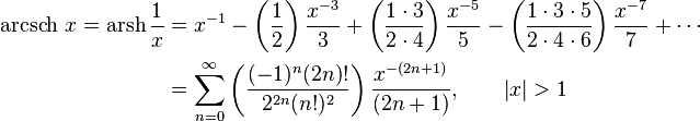
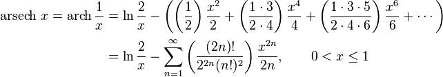
Series expansions[edit]

Expansion series can be obtained for the above functions:

${displaystyle {begin{aligned}operatorname {arsinh} x&=x-left({frac {1}{2}}right){frac {x^{3}}{3}}+left({frac {1cdot 3}{2cdot 4}}right){frac {x^{5}}{5}}-left({frac {1cdot 3cdot 5}{2cdot 4cdot 6}}right){frac {x^{7}}{7}}pm cdots \&=sum _{n=0}^{infty }left({frac {(-1)^{n}(2n)!}{2^{2n}(n!)^{2}}}right){frac {x^{2n+1}}{2n+1}},qquad left|xright|<1end{aligned}}}$

${displaystyle {begin{aligned}operatorname {arcosh} x&=ln(2x)-left(left({frac {1}{2}}right){frac {x^{-2}}{2}}+left({frac {1cdot 3}{2cdot 4}}right){frac {x^{-4}}{4}}+left({frac {1cdot 3cdot 5}{2cdot 4cdot 6}}right){frac {x^{-6}}{6}}+cdots right)\&=ln(2x)-sum _{n=1}^{infty }left({frac {(2n)!}{2^{2n}(n!)^{2}}}right){frac {x^{-2n}}{2n}},qquad left|xright|>1end{aligned}}}$

${displaystyle {begin{aligned}operatorname {artanh} x&=x+{frac {x^{3}}{3}}+{frac {x^{5}}{5}}+{frac {x^{7}}{7}}+cdots \&=sum _{n=0}^{infty }{frac {x^{2n+1}}{2n+1}},qquad left|xright|<1end{aligned}}}$

${displaystyle {begin{aligned}operatorname {arcsch} x=operatorname {arsinh} {frac {1}{x}}&=x^{-1}-left({frac {1}{2}}right){frac {x^{-3}}{3}}+left({frac {1cdot 3}{2cdot 4}}right){frac {x^{-5}}{5}}-left({frac {1cdot 3cdot 5}{2cdot 4cdot 6}}right){frac {x^{-7}}{7}}pm cdots \&=sum _{n=0}^{infty }left({frac {(-1)^{n}(2n)!}{2^{2n}(n!)^{2}}}right){frac {x^{-(2n+1)}}{2n+1}},qquad left|xright|>1end{aligned}}}$

${displaystyle {begin{aligned}operatorname {arsech} x=operatorname {arcosh} {frac {1}{x}}&=ln {frac {2}{x}}-left(left({frac {1}{2}}right){frac {x^{2}}{2}}+left({frac {1cdot 3}{2cdot 4}}right){frac {x^{4}}{4}}+left({frac {1cdot 3cdot 5}{2cdot 4cdot 6}}right){frac {x^{6}}{6}}+cdots right)\&=ln {frac {2}{x}}-sum _{n=1}^{infty }left({frac {(2n)!}{2^{2n}(n!)^{2}}}right){frac {x^{2n}}{2n}},qquad 0<xleq 1end{aligned}}}$

${displaystyle {begin{aligned}operatorname {arcoth} x=operatorname {artanh} {frac {1}{x}}&=x^{-1}+{frac {x^{-3}}{3}}+{frac {x^{-5}}{5}}+{frac {x^{-7}}{7}}+cdots \&=sum _{n=0}^{infty }{frac {x^{-(2n+1)}}{2n+1}},qquad left|xright|>1end{aligned}}}$

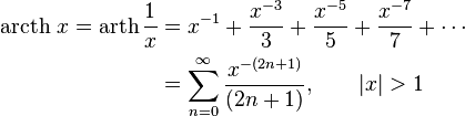
An asymptotic expansion for arsinh is given by

${displaystyle operatorname {arsinh} x=ln(2x)+sum limits _{n=1}^{infty }{left({-1}right)^{n-1}{frac {left({2n-1}right)!!}{2nleft({2n}right)!!}}}{frac {1}{x^{2n}}}}$

Principal values in the complex plane[edit]

As functions of a complex variable, inverse hyperbolic functions are multivalued functions that are analytic, except at a finite number of points. For such a function, it is common to define a principal value, which is a single valued analytic function which coincides with one specific branch of the multivalued function, over a domain consisting of the complex plane in which a finite number of arcs (usually half lines or line segments) have been removed. These arcs are called branch cuts. For specifying the branch, that is, defining which value of the multivalued function is considered at each point, one generally define it at a particular point, and deduce the value everywhere in the domain of definition of the principal value by analytic continuation. When possible, it is better to define the principal value directly—without referring to analytic continuation.

For example, for the square root, the principal value is defined as the square root that has a positive real part. This defines a single valued analytic function, which is defined everywhere, except for non-positive real values of the variables (where the two square roots have a zero real part). This principal value of the square root function is denoted in what follows. Similarly, the principal value of the logarithm, denoted in what follows, is defined as the value for which the imaginary part has the smallest absolute value. It is defined everywhere except for non-positive real values of the variable, for which two different values of the logarithm reach the minimum.

For all inverse hyperbolic functions, the principal value may be defined in terms of principal values of the square root and the logarithm function. However, in some cases, the formulas of § Definitions in terms of logarithms do not give a correct principal value, as giving a domain of definition which is too small and, in one case non-connected.

Principal value of the inverse hyperbolic sine[edit]

The principal value of the inverse hyperbolic sine is given by

$operatorname {arsinh} z=operatorname {Log} (z+{sqrt {z^{2}+1}},),.$

The argument of the square root is a non-positive real number, if and only if z belongs to one of the intervals [i, +i∞) and (−i∞, −i] of the imaginary axis. If the argument of the logarithm is real, then it is positive. Thus this formula defines a principal value for arsinh, with branch cuts [i, +i∞) and (−i∞, −i]. This is optimal, as the branch cuts must connect the singular points i and −i to the infinity.

Principal value of the inverse hyperbolic cosine[edit]

The formula for the inverse hyperbolic cosine given in § Inverse hyperbolic cosine is not convenient, since similar to the principal values of the logarithm and the square root, the principal value of arcosh would not be defined for imaginary z. Thus the square root has to be factorized, leading to

operatorname {arcosh} z=operatorname {Log} (z+{sqrt {z+1}}{sqrt {z-1}},),.

The principal values of the square roots are both defined, except if z belongs to the real interval (−∞, 1]. If the argument of the logarithm is real, then z is real and has the same sign. Thus, the above formula defines a principal value of arcosh outside the real interval (−∞, 1], which is thus the unique branch cut.

Principal values of the inverse hyperbolic tangent and cotangent[edit]

The formulas given in § Definitions in terms of logarithms suggests

${displaystyle {begin{aligned}operatorname {artanh} z&={frac {1}{2}}operatorname {Log} left({frac {1+z}{1-z}}right)\operatorname {arcoth} z&={frac {1}{2}}operatorname {Log} left({frac {z+1}{z-1}}right)end{aligned}}}$

for the definition of the principal values of the inverse hyperbolic tangent and cotangent. In these formulas, the argument of the logarithm is real if and only if z is real. For artanh, this argument is in the real interval (−∞, 0], if z belongs either to (−∞, −1] or to [1, ∞). For arcoth, the argument of the logarithm is in (−∞, 0], if and only if z belongs to the real interval [−1, 1].

Therefore, these formulas define convenient principal values, for which the branch cuts are (−∞, −1] and [1, ∞) for the inverse hyperbolic tangent, and [−1, 1] for the inverse hyperbolic cotangent.

In view of a better numerical evaluation near the branch cuts, some authors^{[citation needed]} use the following definitions of the principal values, although the second one introduces a removable singularity at z = 0. The two definitions of differ for real values of with . The ones of differ for real values of with .

${displaystyle {begin{aligned}operatorname {artanh} z&={tfrac {1}{2}}operatorname {Log} left({1+z}right)-{tfrac {1}{2}}operatorname {Log} left({1-z}right)\operatorname {arcoth} z&={tfrac {1}{2}}operatorname {Log} left({1+{frac {1}{z}}}right)-{tfrac {1}{2}}operatorname {Log} left({1-{frac {1}{z}}}right)end{aligned}}}$

Principal value of the inverse hyperbolic cosecant[edit]

For the inverse hyperbolic cosecant, the principal value is defined as

$operatorname {arcsch} z=operatorname {Log} left({frac {1}{z}}+{sqrt {{frac {1}{z^{2}}}+1}},right)$

It is defined when the arguments of the logarithm and the square root are not non-positive real numbers. The principal value of the square root is thus defined outside the interval [−i, i] of the imaginary line. If the argument of the logarithm is real, then z is a non-zero real number, and this implies that the argument of the logarithm is positive.

Thus, the principal value is defined by the above formula outside the branch cut, consisting of the interval [−i, i] of the imaginary line.

For z = 0, there is a singular point that is included in the branch cut.

Principal value of the inverse hyperbolic secant[edit]

Here, as in the case of the inverse hyperbolic cosine, we have to factorize the square root. This gives the principal value

${displaystyle operatorname {arsech} z=operatorname {Log} left({frac {1}{z}}+{sqrt {{frac {1}{z}}+1}},{sqrt {{frac {1}{z}}-1}}right).}$

If the argument of a square root is real, then z is real, and it follows that both principal values of square roots are defined, except if z is real and belongs to one of the intervals (−∞, 0] and [1, +∞). If the argument of the logarithm is real and negative, then z is also real and negative. It follows that the principal value of arsech is well defined, by the above formula outside two branch cuts, the real intervals (−∞, 0] and [1, +∞).

For z = 0, there is a singular point that is included in one of the branch cuts.

Graphical representation[edit]

In the following graphical representation of the principal values of the inverse hyperbolic functions, the branch cuts appear as discontinuities of the color. The fact that the whole branch cuts appear as discontinuities, shows that these principal values may not be extended into analytic functions defined over larger domains. In other words, the above defined branch cuts are minimal.

Inverse hyperbolic functions in the complex z-plane: the colour at each point in the plane represents the complex value of the respective function at that point

References[edit]

^ For example: Weltner, Klaus; et al. (2014) [2009]. Mathematics for Physicists and Engineers (2nd ed.). Springer. ISBN 978-364254124-7. Durán, Mario (2012). Mathematical methods for wave propagation in science and engineering. Vol. 1. Ediciones UC. p. 89. ISBN 9789561413146.
^ Birman, Graciela S.; Nomizu, Katsumi (1984). «Trigonometry in Lorentzian Geometry». American Mathematical Monthly. 91 (9): 543–549. JSTOR 2323737.
^ Sobczyk, Garret (1995). «The hyperbolic number plane». College Mathematics Journal. 26 (4): 268–280.
^
Weisstein, Eric W. «Inverse Hyperbolic Functions». Wolfram Mathworld. Retrieved 2020-08-30. «Inverse hyperbolic functions». Encyclopedia of Mathematics. Retrieved 2020-08-30.
^ Press, W.H.; Teukolsky, S.A.; Vetterling, WT; Flannery, B.P. (1992). «§ 5.6. Quadratic and Cubic Equations». Numerical Recipes in FORTRAN (2nd ed.). Cambridge University Press. ISBN 0-521-43064-X. Woodhouse, N.M.J. (2003). Special Relativity. Springer. p. 71. ISBN 1-85233-426-6.
^ Gullberg, Jan (1997). Mathematics: From the Birth of Numbers. W. W. Norton. p. 539. ISBN 039304002X. Another form of notation, arcsinh x, arccosh x, etc., is a practice to be condemned as these functions have nothing whatever to do with arc, but with area, as is demonstrated by their full Latin names, ¶ arsinh area sinus hyperbolicus ¶ arcosh area cosinus hyperbolicus, etc. Zeidler, Eberhard; Hackbusch, Wolfgang; Schwarz, Hans Rudolf (2004). «§ 0.2.13 The inverse hyperbolic functions». Oxford Users’ Guide to Mathematics. Translated by Hunt, Bruce. Oxford University Press. p. 68. ISBN 0198507631. The Latin names for the inverse hyperbolic functions are area sinus hyperbolicus, area cosinus hyperbolicus, area tangens hyperbolicus and area cotangens hyperbolicus (of x)….. Zeidler & al. use the notations arsinh, etc.; note that the quoted Latin names are back-formations, invented long after Neo-Latin ceased to be in common use in mathematical literature. Bronshtein, Ilja N.; Semendyayev, Konstantin A.; Musiol, Gerhard; Heiner, Mühlig (2007). «§ 2.10: Area Functions». Handbook of Mathematics (5th ed.). Springer. p. 91. doi:10.1007/978-3-540-72122-2. ISBN 3540721215. The area functions are the inverse functions of the hyperbolic functions, i.e., the inverse hyperbolic functions. The functions sinh x, tanh x, and coth x are strictly monotone, so they have unique inverses without any restriction; the function cosh x has two monotonic intervals so we can consider two inverse functions. The name area refers to the fact that the geometric definition of the functions is the area of certain hyperbolic sectors … Bacon, Harold Maile (1942). Differential and Integral Calculus. McGraw-Hill. p. 203.
^ «Identities with inverse hyperbolic and trigonometric functions». math stackexchange. stackexchange. Retrieved 3 November 2016.

Bibliography[edit]

Herbert Busemann and Paul J. Kelly (1953) Projective Geometry and Projective Metrics, page 207, Academic Press.

External links[edit]

«Inverse hyperbolic functions», Encyclopedia of Mathematics, EMS Press, 2001 [1994]

Источник

ГИПЕРБОЛИЧЕСКИЕ
ФУНКЦИИ

ОБРАТНЫЕ
ГИПЕРБОЛИЧЕСКИЕ ФУНКЦИИ

ГИПЕРБОЛИЧЕСКИЕ
ФУНКЦИИ

Гиперболические
функции

Определение

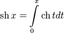
Гиперболические
функции задаются следующими формулами:

гиперболический
синус:

(в
англоязычной литературе обозначается
)

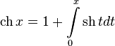
гиперболический
косинус:

(в
англоязычной литературе обозначается
)

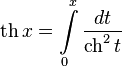
гиперболический
тангенс:

(в
англоязычной литературе обозначается
)

гиперболический
котангенс:

гиперболические
секанс и косеканс:

Свойства

Связь
с тригонометрическими функциями:

Гиперболические
функции выражаются через тригонометрические
функции от мнимого
аргумента.

Важные
соотношения:

Чётность:
Формулы
сложения:
Формулы
двойного угла:
Формулы
кратных углов:
Произведения
Суммы
Формулы
понижения степени
Производные:
Интегралы:

Неравенства:

Для
всех
выполняется:

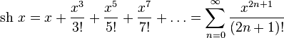
Разложение
в степенные ряды:

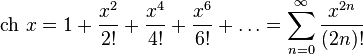
(Ряд
Лорана)

Здесь
—
числа
Бернулли.

Графики:

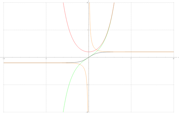
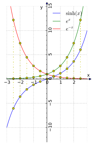
sh(x),
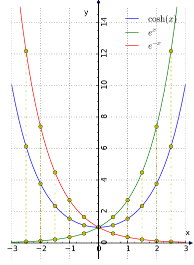
ch(x),
th(x),
cth(x)

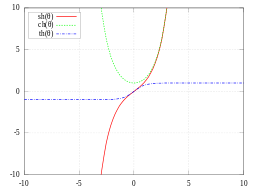
sh,
ch
и th

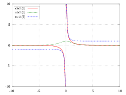
csch,
sech
и cth

Обратные
гиперболические функции

—
обратный
гиперболический синус, гиперболический
арксинус, ареасинус:

—
обратный
гиперболический косинус, гиперболический
арккосинус, ареакосинус.

—
обратный
гиперболический тангенс, гиперболический
арктангенс, ареатангенс.

—
обратный
гиперболический котангенс, гиперболический
арккотангенс, ареакотангенс.

—
обратный
гиперболический секанс, гиперболический
арксеканс, ареасеканс.

—
обратный
гиперболический косеканс, гиперболический
арккосеканс, ареакосеканс.

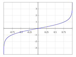
Графики:

arsh(x),
arch(x),
arth(x),
arcth(x)

Связь
между некоторыми обратными гиперболическими
и обратными тригонометрическими
функциями:

где
i
— мнимая единица.

Эти
функции имеют следующее разложение в
ряд:

ОБРАТНЫЕ
ГИПЕРБОЛИЧЕСКИЕ ФУНКЦИИ

Обратные
гиперболические функции

Название функции	Обозначение в русской литературе	Обозначение в английской литературе
ареасинус	arsh	arsinh, sinh⁻¹
ареакосинус	arch	arcosh, cosh⁻¹
ареатангенс	arth	artanh, tanh⁻¹
ареакотангенс	arcth	arcotanh, cotanh⁻¹
ареасеканс	arsech	arsech, sech⁻¹
ареакосеканс	arcsch	arcsch, csch⁻¹

Определения
функций

Гиперболический
ареасинус для действительного аргумента

Гиперболический
ареакосинус для действительного
аргумента

Гиперболический
ареатангенс для действительного
аргумента

Гиперболический
ареакотангенс для действительного
аргумента

Гиперболический
ареасеканс для действительного аргумента

Гиперболический
ареакосеканс для действительного
аргумента

В
комплексной
плоскости функции можно определить
формулами:

Гиперболический
ареасинус:

Гиперболический
ареакосинус:

Гиперболический
ареатангенс:

Гиперболический
ареакотангенс:

Гиперболический
ареасеканс:

Гиперболический
ареакосеканс:

Разложение
в ряд

Обратные
гиперболические функции можно разложить
в ряды:

Асимптотическое
разложение arsh x
даётся формулой:

Производные

Для
действительных x:

Пример
дифференцирования: если θ = arsh x,
то:

Комбинация
гиперболических и обратных гиперболических
функций

Дополнительные
формулы

Соседние файлы в предмете [НЕСОРТИРОВАННОЕ]

Источник

Обра́тные гиперболи́ческие фу́нкции (известные также как а̀реафу́нкции или ареа-функции) — семейство элементарных функций, определяющихся как обратные функции к гиперболическим функциям. Эти функции определяют площадь сектора единичной гиперболы x² − y² = 1 аналогично тому, как обратные тригонометрические функции определяют длину дуги единичной окружности x² + y² = 1. Для этих функций часто используются обозначения arcsinh, arcsh, arccosh, arcch и т.д., хотя такие обозначения являются, строго говоря, ошибочными, так как префикс arc является сокращением от arcus (дуга) и потому относится только к обратным тригонометрическим функциям, тогда как ar обозначает area — площадь. Более правильными являются обозначения arsinh, arsh и т.д. и названия обратный гиперболический синус, ареасинус и т.д. Также применяют^[1] названия гиперболический ареасинус, гиперболический ареакосинус и т.д., но слово «гиперболический» здесь является лишним, поскольку на принадлежность функции семейству обратных гиперболических функций однозначно указывает префикс «ареа». Иногда названия соответствующих функций записывают через дефис: ареа-синус, ареа-косинус и т.д.

В комплексной плоскости гиперболические функции являются периодическими, а обратные им функции — многозначными. Поэтому подобно обратным тригонометрическим функциям обозначения ареафункций принято записывать с большой буквы, если подразумевается множество значений функции (логарифм в соответствующем определении функции также понимается как общее значение логарифма, обозначаемое Ln). С маленькой буквы записываются главные значения соответствующих функций.

В русской литературе обозначения большинства прямых и обратных гиперболических функций (так же как и части тригонометрических) отличаются от английских обозначений.

Название функции	Обозначение в русской литературе	Обозначение в английской литературе
ареасинус	arsh	arsinh, sinh⁻¹
ареакосинус	arch	arcosh, cosh⁻¹
ареатангенс	arth	artanh, tanh⁻¹
ареакотангенс	arcth	arcoth, coth⁻¹
ареасеканс	arsch, arsech	arsech, sech⁻¹
ареакосеканс	arcsch	arcsch, csch⁻¹

Определения функций

Ареасинус для действительного аргумента

Ареакосинус для действительного аргумента

Ареатангенс для действительного аргумента

Ареакотангенс для действительного аргумента

Ареасеканс для действительного аргумента

Ареакосеканс для действительного аргумента

В комплексной плоскости главные значения функций можно определить формулами:

ареасинус

[math]displaystyle{
operatorname{arsh}, z = ln(z + sqrt{z^2 + 1} ,); }[/math]

ареакосинус

[math]displaystyle{ operatorname{arch}, z = ln(z + sqrt{z^2-1}); }[/math]

ареатангенс

[math]displaystyle{ operatorname{arth}, z = tfrac12lnleft(frac{1+z}{1-z}right); }[/math]

ареакотангенс

[math]displaystyle{ operatorname{arcth}, z = tfrac12lnleft(frac{z+1}{z-1}right); }[/math]

ареасеканс

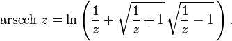
[math]displaystyle{ operatorname{arsech}, z = lnleft( frac{1}{z} + sqrt{ frac{1}{z^2} — 1 }right); }[/math]

ареакосеканс

[math]displaystyle{ operatorname{arcsch}, z = lnleft( frac{1}{z} + sqrt{ frac{1}{z^2} +1 } ,right). }[/math]

Квадратными корнями в этих формулах являются главные значения квадратного корня (то есть [math]displaystyle{ sqrt{z} = sqrt{r} , e^{i varphi / 2}, }[/math] если представить комплексное число z как [math]displaystyle{ z=r e^{i varphi} }[/math] при [math]displaystyle{ -pi lt varphi le pi }[/math]), а логарифмические функции являются функциями комплексной переменной. Для действительных аргументов можно осуществить некоторые упрощения, например [math]displaystyle{ sqrt{x+1}sqrt{x-1}=sqrt{x^2-1}, }[/math] которые не всегда верны для главных значений квадратных корней.

Разложение в ряд

Обратные гиперболические функции можно разложить в ряды:

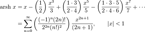
[math]displaystyle{ begin{align}operatorname{arsh}, x & = x — left( frac {1} {2} right) frac {x^3} {3} + left( frac {1 cdot 3} {2 cdot 4} right) frac {x^5} {5} — left( frac {1 cdot 3 cdot 5} {2 cdot 4 cdot 6} right) frac {x^7} {7} +cdots \
& = sum_{n=0}^infty left( frac {(-1)^n(2n-1)!!} {(2n)!!} right) frac {x^{2n+1}} {(2n+1)} , qquad left| x right| lt 1. end{align} }[/math]

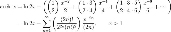
[math]displaystyle{ begin{align}operatorname{arch}, x & = ln 2x — left( left( frac {1} {2} right) frac {x^{-2}} {2} + left( frac {1 cdot 3} {2 cdot 4} right) frac {x^{-4}} {4} + left( frac {1 cdot 3 cdot 5} {2 cdot 4 cdot 6} right) frac {x^{-6}} {6} +cdots right) \
& = ln 2x — sum_{n=1}^infty left( frac {(2n)!} {2^{2n}(n!)^2} right) frac {x^{-2n}} {(2n)} , qquad x gt 1. end{align} }[/math]

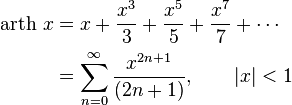
[math]displaystyle{ begin{align}operatorname{arth}, x & = x + frac {x^3} {3} + frac {x^5} {5} + frac {x^7} {7} +cdots \
& = sum_{n=0}^infty frac {x^{2n+1}} {(2n+1)} , qquad left| x right| lt 1. end{align} }[/math]

[math]displaystyle{ begin{align}operatorname{arcsch}, x = operatorname{arsh} frac1x & = x^{-1} — left( frac {1} {2} right) frac {x^{-3}} {3} + left( frac {1 cdot 3} {2 cdot 4} right) frac {x^{-5}} {5} — left( frac {1 cdot 3 cdot 5} {2 cdot 4 cdot 6} right) frac {x^{-7}} {7} +cdots \
& = sum_{n=0}^infty left( frac {(-1)^n(2n)!} {2^{2n}(n!)^2} right) frac {x^{-(2n+1)}} {(2n+1)} , qquad left| x right| gt 1. end{align} }[/math]

[math]displaystyle{ begin{align}operatorname{arsech}, x = operatorname{arch} frac1x & = ln frac{2}{x} — left( left( frac {1} {2} right) frac {x^{2}} {2} + left( frac {1 cdot 3} {2 cdot 4} right) frac {x^{4}} {4} + left( frac {1 cdot 3 cdot 5} {2 cdot 4 cdot 6} right) frac {x^{6}} {6} +cdots right) \
& = ln frac{2}{x} — sum_{n=1}^infty left( frac {(2n)!} {2^{2n}(n!)^2} right) frac {x^{2n}} {2n} , qquad 0 lt x le 1. end{align} }[/math]

[math]displaystyle{ begin{align}operatorname{arcth}, x = operatorname{arth} frac1x & = x^{-1} + frac {x^{-3}} {3} + frac {x^{-5}} {5} + frac {x^{-7}} {7} +cdots \
& = sum_{n=0}^infty frac {x^{-(2n+1)}} {(2n+1)} , qquad left| x right| gt 1. end{align} }[/math]

Асимптотическое разложение arsh x даётся формулой

[math]displaystyle{ operatorname{arsh}, x = ln 2x + sumlimits_{n = 1}^infty {left( { — 1} right)^{n — 1} frac{{left( {2n — 1} right)!!}}{{2nleft( {2n} right)!!}}} frac{1}{{x^{2n} }}. }[/math]

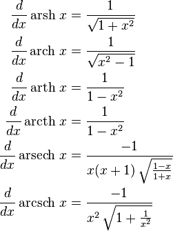
Производные

Функция [math]displaystyle{ f(x) }[/math]	Производная [math]displaystyle{ f'(x) }[/math]	Примечание
[math]displaystyle{ mathrm{arsh} x }[/math]	[math]displaystyle{ frac{1}{sqrt{x^2 + 1}} }[/math]	Доказательство [math]displaystyle{ (arsh (x))’ = (ln{(x + sqrt{x^2 + 1})})’ = frac{1}{x + sqrt{x^2 + 1}} cdot (x + sqrt{x^2 + 1})’ = frac{1}{x + sqrt{x^2 + 1}} cdot ((x)’ + (sqrt{x^2 + 1})’) = frac{1}{x + sqrt{x^2 + 1}} cdot (1 + (sqrt{x^2 + 1})’) = frac{1}{x + sqrt{x^2 + 1}} cdot (1 + frac{1}{2sqrt{x^2 + 1}} cdot (x^2 + 1)’) = frac{1}{x + sqrt{x^2 + 1}} cdot (1 + frac{2x}{2sqrt{x^2 + 1}}) = frac{1}{x + sqrt{x^2 + 1}} cdot (frac{x + sqrt{x^2 + 1}}{sqrt{x^2 + 1}}) = frac{x + sqrt{x^2 + 1}}{(x + sqrt{x^2 + 1}) cdot (sqrt{x^2 + 1})} = frac{1}{sqrt{x^2 + 1}} }[/math]
[math]displaystyle{ mathrm{arch} x }[/math]	[math]displaystyle{ frac{1}{sqrt{x^2 — 1}} }[/math]	Доказательство [math]displaystyle{ (arch (x))’ = (ln{(x + sqrt{x^2 — 1})})’ = frac{1}{x + sqrt{x^2 — 1}} cdot (x + sqrt{x^2 — 1})’ = frac{1}{x + sqrt{x^2 — 1}} cdot ((x)’ + (sqrt{x^2 — 1})’) = frac{1}{x + sqrt{x^2 — 1}} cdot (1 + (sqrt{x^2 — 1})’) = frac{1}{x + sqrt{x^2 — 1}} cdot (1 + frac{1}{2sqrt{x^2 — 1}} cdot (x^2 — 1)’) = frac{1}{x + sqrt{x^2 — 1}} cdot (1 + frac{2x}{2sqrt{x^2 — 1}}) = frac{1}{x + sqrt{x^2 — 1}} cdot (frac{x + sqrt{x^2 — 1}}{sqrt{x^2 — 1}}) = frac{x + sqrt{x^2 — 1}}{(x + sqrt{x^2 — 1}) cdot (sqrt{x^2 — 1})} = frac{1}{sqrt{x^2 — 1}} }[/math]
[math]displaystyle{ mathrm{arth} x }[/math]	[math]displaystyle{ frac{1}{1 — x^2} }[/math]	Доказательство [math]displaystyle{ ({displaystyle mathrm {arth} x})’ = biggl(frac{1}{2} cdot lnbiggl(frac{1+x}{1-x}biggl)biggl)’ = frac{1}{2} cdot frac{1-x}{1+x} cdot biggl(frac{1+x}{1-x}biggl)’ = frac{1}{2} cdot frac{1-x}{1+x} cdot frac{(1+x)'(1-x) — (1+x)(1-x)’}{(1-x)^2} = frac{1}{2} cdot frac{1-x}{1+x} cdot frac{2}{(1-x)^2} = frac{1}{1-x^2} }[/math]
[math]displaystyle{ mathrm{arcth} x }[/math]	[math]displaystyle{ frac{1}{1 — x^2} }[/math]	Доказательство [math]displaystyle{ ({displaystyle mathrm {arcth} x})’ = biggl(frac{1}{2} cdot lnbiggl(frac{x+1}{x-1}biggl)biggl)’ = frac{1}{2} cdot frac{x-1}{x+1} cdot biggl(frac{x+1}{x-1}biggl)’ = frac{1}{2} cdot frac{x-1}{x+1} cdot frac{(x+1)'(x-1) — (x+1)(x-1)’}{(x-1)^2} = frac{1}{2} cdot frac{x-1}{x+1} cdot frac{-2}{(x-1)^2} = frac{1}{1-x^2} }[/math]
[math]displaystyle{ mathrm{arsech} x }[/math]	[math]displaystyle{ -frac{1}{x(x+1)sqrt{frac{1-x}{1+x}}} }[/math]
[math]displaystyle{ mathrm{arcsch} x }[/math]	[math]displaystyle{ -frac{1}{x(x+1)sqrt{1 + frac{1}{x^2}}} }[/math]

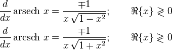
Для действительных x:

[math]displaystyle{
begin{align}
frac{d}{dx} operatorname{arsech}, x & {}= mp frac{1}{x,sqrt{1-x^2}}; qquad Re{x} gtrless 0.\
frac{d}{dx} operatorname{arcsch}, x & {}= mp frac{1}{x,sqrt{1+x^2}}; qquad Re{x} gtrless 0.
end{align} }[/math]

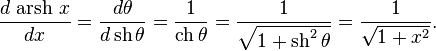
Пример дифференцирования: если θ = arsh x, то:

[math]displaystyle{ frac{d,operatorname{arsh}, x}{dx} = frac{d theta}{d operatorname{sh} theta} = frac{1} {operatorname{ch} theta} = frac{1} {sqrt{1+operatorname{sh}^2 theta}} = frac{1}{sqrt{1+x^2}}. }[/math]

Комбинация гиперболических и обратных гиперболических функций

[math]displaystyle{ begin{align}
&operatorname{sh}(operatorname{arch},x) = sqrt{x^{2} — 1}, quad quad |x| gt 1; \
&operatorname{sh}(operatorname{arth},x) = frac{x}{sqrt{1-x^{2}}}, quad quad -1 lt x lt 1; \
&operatorname{ch}(operatorname{arsh},x) = sqrt{1+x^{2}}; \
&operatorname{ch}(operatorname{arth},x) = frac{1}{sqrt{1-x^{2}}}, quad quad -1 lt x lt 1; \
&operatorname{th}(operatorname{arsh},x) = frac{x}{sqrt{1+x^{2}}}; \
&operatorname{th}(operatorname{arch},x) = frac{sqrt{x^{2} — 1}}{x}, quad quad |x| gt 1.
end{align} }[/math]

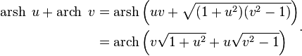
Дополнительные формулы

[math]displaystyle{ operatorname{arsh} ;u pm operatorname{arsh} ;v = operatorname{arsh} left(u sqrt{1 + v^2} pm v sqrt{1 + u^2}right). }[/math]

[math]displaystyle{ operatorname{arch} ;u pm operatorname{arch} ;v = operatorname{arch} left(u v pm sqrt{(u^2 — 1) (v^2 — 1)}right). }[/math]

[math]displaystyle{ operatorname{arth} ;u pm operatorname{arth} ;v = operatorname{arth} left( frac{u pm v}{1 pm uv} right). }[/math]

[math]displaystyle{ begin{align}operatorname{arsh} ;u + operatorname{arch} ;v & = operatorname{arsh} left(u v + sqrt{(1 + u^2) (v^2 — 1)}right) \
& = operatorname{arch} left(v sqrt{1 + u^2} + u sqrt{v^2 — 1}right). end{align} }[/math]

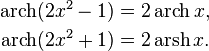
[math]displaystyle{ begin{align}
2operatorname{arch} x &=operatorname{arch}(2x^2-1), &quadquad xgeq 1; \
4operatorname{arch} x &=operatorname{arch}(8x^4-8x^2+1), &quadquad xgeq 1; \
2operatorname{arsh} x &= operatorname{arch}(2x^2+1), &quadquad xgeq 0; \
4operatorname{arsh} x &= operatorname{arch}(8x^4+8x^2+1), &quadquad xgeq 0. \
end{align} }[/math]

См. также

Гиперболические функции
Обратные тригонометрические функции
Таблица интегралов обратных гиперболических функций

Источники

↑ М.Я. Выгодский. Справочник по высшей математике. — Наука, 1963. — С. 594. — 873 с.

Herbert Busemann, Paul J. Kelly (1953) Projective Geometry and Projective Metrics, с. 207, Academic Press.

Ссылки

Inverse hyperbolic functions на сайте MathWorld
Inverse hyperbolic functions

Источник

Обратные гиперболические функции — определяются как обратные функции к гиперболическим функциям. Эти функции определяют площадь сектора единичной гиперболы x² − y² = 1 аналогично тому, как обратные тригонометрические функции определяют длину дуги единичной окружности x² + y² = 1. Для этих функций часто используются обозначення arcsinh, arcsh, arccosh, arcch и т. д., хотя такое обозначение является в общем случае ошибочным, так как arc является сокращением от arcus — дуга, тогда как префикс ar обозначает area — площадь. Более правильными являются обозначения arsinh, arsh и т. д. и названия гиперболический ареасинус, гиперболический ареакосинус и т. д.

Содержание

1 Определения функций
2 Разложение в ряд
3 Производные
4 Комбинация гиперболических и обратных гиперболических функций
5 Дополнительные формулы
6 См. также
7 Источники
8 Ссылки

Определения функций

Гиперболический ареасинус для действительного аргумента

Гиперболический ареакосинус для действительного аргумента

Гиперболический ареатангенс для действительного аргумента

Гиперболический ареакотангенс для действительного аргумента

Гиперболический ареасеканс для действительного аргумента

Гиперболический ареакосеканс для действительного аргумента

В комплексной плоскости функции можно определить формулами:

Гиперболический ареасинус

$operatorname{arsinh}, z = ln(z + sqrt{z^2 + 1} ,),$

Гиперболический ареакосинус

operatorname{arcosh}, z = ln(z + sqrt{z+1} sqrt{z-1} ,),

Гиперболический ареатангенс

$operatorname{artanh}, z = tfrac12ln(frac{1+z}{1-z}).$

Гиперболический ареакотангенс

$operatorname{arcoth}, z = tfrac12ln(frac{z+1}{z-1}).$

Гиперболический ареасеканс

$operatorname{arcsch}, z = lnleft( frac{1}{z} + sqrt{ frac{1}{z^2} +1 } ,right),$

Гиперболический ареакосеканс

$operatorname{arsech}, z = lnleft( frac{1}{z} + sqrt{ frac{1}{z} + 1 } , sqrt{ frac{1}{z} -1 } ,right).$

Квадратными корнями в этих формулах являются главные значения квадратного корня и логарифмические функции являются функциями комплексной переменной. Для действительных аргументов можно осуществить некоторые упрощения, например $sqrt{x+1}sqrt{x-1}=sqrt{x^2-1}$ , которые не всегда верно для главных значений квадратных корней.

Разложение в ряд

Обратные гиперболические функции можно разложить в ряды:

$begin{align}operatorname{arsinh}, x & = x - left( frac {1} {2} right) frac {x^3} {3} + left( frac {1 cdot 3} {2 cdot 4} right) frac {x^5} {5} - left( frac {1 cdot 3 cdot 5} {2 cdot 4 cdot 6} right) frac {x^7} {7} +cdots \ & = sum_{n=0}^infty left( frac {(-1)^n(2n)!} {2^{2n}(n!)^2} right) frac {x^{2n+1}} {(2n+1)} , qquad left| x right| < 1 end{align}$

$begin{align}operatorname{arcosh}, x & = ln 2x - left( left( frac {1} {2} right) frac {x^{-2}} {2} + left( frac {1 cdot 3} {2 cdot 4} right) frac {x^{-4}} {4} + left( frac {1 cdot 3 cdot 5} {2 cdot 4 cdot 6} right) frac {x^{-6}} {6} +cdots right) \ & = ln 2x - sum_{n=1}^infty left( frac {(2n)!} {2^{2n}(n!)^2} right) frac {x^{-2n}} {(2n)} , qquad x > 1 end{align}$

$begin{align}operatorname{artanh}, x & = x + frac {x^3} {3} + frac {x^5} {5} + frac {x^7} {7} +cdots \ & = sum_{n=0}^infty frac {x^{2n+1}} {(2n+1)} , qquad left| x right| < 1 end{align}$

$begin{align}operatorname{arcsch}, x = operatorname{arsinh} frac1x & = x^{-1} - left( frac {1} {2} right) frac {x^{-3}} {3} + left( frac {1 cdot 3} {2 cdot 4} right) frac {x^{-5}} {5} - left( frac {1 cdot 3 cdot 5} {2 cdot 4 cdot 6} right) frac {x^{-7}} {7} +cdots \ & = sum_{n=0}^infty left( frac {(-1)^n(2n)!} {2^{2n}(n!)^2} right) frac {x^{-(2n+1)}} {(2n+1)} , qquad left| x right| > 1 end{align}$

$begin{align}operatorname{arsech}, x = operatorname{arcosh} frac1x & = ln frac{2}{x} - left( left( frac {1} {2} right) frac {x^{2}} {2} + left( frac {1 cdot 3} {2 cdot 4} right) frac {x^{4}} {4} + left( frac {1 cdot 3 cdot 5} {2 cdot 4 cdot 6} right) frac {x^{6}} {6} +cdots right) \ & = ln frac{2}{x} - sum_{n=1}^infty left( frac {(2n)!} {2^{2n}(n!)^2} right) frac {x^{2n}} {2n} , qquad 0 < x le 1 end{align}$

$begin{align}operatorname{arcoth}, x = operatorname{artanh} frac1x & = x^{-1} + frac {x^{-3}} {3} + frac {x^{-5}} {5} + frac {x^{-7}} {7} +cdots \ & = sum_{n=0}^infty frac {x^{-(2n+1)}} {(2n+1)} , qquad left| x right| > 1 end{align}$

Asymptotic expansion for the arsinh x is given by

$operatorname{arsinh}, x = ln 2x + sumlimits_{n = 1}^infty {left( { - 1} right)^{n - 1} frac{{left( {2n - 1} right)!!}}{{2nleft( {2n} right)!!}}} frac{1}{{x^{2n} }}$

Производные

$begin{align} frac{d}{dx} operatorname{arsinh}, x & {}= frac{1}{sqrt{1+x^2}}\ frac{d}{dx} operatorname{arcosh}, x & {}= frac{1}{sqrt{x^2-1}}\ frac{d}{dx} operatorname{artanh}, x & {}= frac{1}{1-x^2}\ frac{d}{dx} operatorname{arcoth}, x & {}= frac{1}{1-x^2}\ frac{d}{dx} operatorname{arsech}, x & {}= frac{-1}{x(x+1),sqrt{frac{1-x}{1+x}}}\ frac{d}{dx} operatorname{arcsch}, x & {}= frac{-1}{x^2,sqrt{1+frac{1}{x^2}}}\ end{align}$

Для действительных x:

$begin{align} frac{d}{dx} operatorname{arsech}, x & {}= frac{mp 1}{x,sqrt{1-x^2}}; qquad Re{x} gtrless 0\ frac{d}{dx} operatorname{arcsch}, x & {}= frac{mp 1}{x,sqrt{1+x^2}}; qquad Re{x} gtrless 0 end{align}$

Пример дифференцирования: если θ = arsinh x, то:

$frac{d,operatorname{arsinh}, x}{dx} = frac{d theta}{d sinh theta} = frac{1} {cosh theta} = frac{1} {sqrt{1+sinh^2 theta}} = frac{1}{sqrt{1+x^2}}$

Комбинация гиперболических и обратных гиперболических функций

$begin{align} &operatorname{sinh}(operatorname{arcosh},x) = sqrt{x^{2} - 1} quad text{for} quad |x| > 1 \ &operatorname{sinh}(operatorname{artanh},x) = frac{x}{sqrt{1-x^{2}}} quad text{for} quad -1 < x < 1 \ &operatorname{cosh}(operatorname{arsinh},x) = sqrt{1+x^{2}} \ &operatorname{cosh}(operatorname{artanh},x) = frac{1}{sqrt{1-x^{2}}} quad text{for} quad -1 < x < 1 \ &operatorname{tanh}(operatorname{arsinh},x) = frac{x}{sqrt{1+x^{2}}} \ &operatorname{tanh}(operatorname{arcosh},x) = frac{sqrt{x^{2} - 1}}{x} quad text{for} quad |x| > 1 end{align}$

Дополнительные формулы

$operatorname{arsinh} ;u pm operatorname{arsinh} ;v = operatorname{arsinh} left(u sqrt{1 + v^2} pm v sqrt{1 + u^2}right)$

$operatorname{arcosh} ;u pm operatorname{arcosh} ;v = operatorname{arcosh} left(u v pm sqrt{(u^2 - 1) (v^2 - 1)}right)$

$operatorname{artanh} ;u pm operatorname{artanh} ;v = operatorname{artanh} left( frac{u pm v}{1 pm uv} right)$

$begin{align}operatorname{arsinh} ;u + operatorname{arcosh} ;v & = operatorname{arsinh} left(u v + sqrt{(1 + u^2) (v^2 - 1)}right) \ & = operatorname{arcosh} left(v sqrt{1 + u^2} + u sqrt{v^2 - 1}right) end{align}$

$operatorname{arcosh}(2x^2-1)=2operatorname{arcosh}(x)$

См. также

Гиперболические функции
Обратные тригонометрические функции
Таблица интегралов обратных гиперболических функций

Источники

Herbert Busemann, Paul J. Kelly (1953) Projective Geometry and Projective Metrics, с. 207, Academic Press.

Ссылки

Inverse hyperbolic functions на сайте MathWorld
Inverse hyperbolic functions

Источник

Луч, проходящий через единичную гиперболу в точке , где вдвое больше площади между лучом, гиперболой и осью. $scriptstyle х ^ {2} - y ^ {2} = 1$

Обратные гиперболические функции

В математике , то обратные гиперболические функции являются обратными функциями этих гиперболических функций .

Для данного значения гиперболической функции соответствующая обратная гиперболическая функция обеспечивает соответствующий гиперболический угол . Размер гиперболического угла равен площади соответствующего гиперболического сектора гиперболы xy = 1 , или в два раза больше площади соответствующего сектора единичной гиперболы x ² — y ² = 1 , точно так же, как круговой угол в два раза больше. площадь кругового сектора на единичной окружности . Некоторые авторы назвали обратные гиперболические функции « функциями площади », чтобы реализовать гиперболические углы.

Гиперболические функции встречаются при вычислении углов и расстояний в гиперболической геометрии . Это также происходит в решениях многих линейных дифференциальных уравнений (таких как уравнение, определяющее цепную связь ), кубических уравнений и уравнения Лапласа в декартовых координатах . Уравнения Лапласа важны во многих областях физики , включая теорию электромагнетизма , теплопередачу , гидродинамику и специальную теорию относительности .

Обозначение

Наиболее распространены сокращения, указанные в стандарте ISO 80000-2 . Они состоят из ар- и аббревиатуры соответствующей гиперболической функции (например, арсинх, аркош).

Тем не менее, дуговой следует соответствующей гиперболической функция (например, arcsinh, arccosh) также часто наблюдается, по аналогии с номенклатурой для обратных тригонометрических функций . Это неправильное употребление, поскольку префикс arc — это сокращение от arcus , а префикс ar означает площадь ; гиперболические функции не имеют прямого отношения к дугам.

Другие авторы предпочитают использовать обозначения arg sinh, argcosh, argtanh и т. Д., Где префикс arg является сокращением латинского argumentsum . В информатике это часто сокращается до asinh .

Обозначения sinh ⁻¹ ( x ) , ch ⁻¹ ( x ) и т. Д. Также используются, несмотря на то, что необходимо проявлять осторожность, чтобы избежать неправильной интерпретации надстрочного индекса −1 как степени, в отличие от сокращения для обозначения обратная функция (например, ch ⁻¹ ( x ) по сравнению с ch ( x ) ⁻¹ ).

Определения в терминах логарифмов

Поскольку гиперболические функции являются рациональными функциями от e ^x , числитель и знаменатель которых имеют степень не выше двух, эти функции могут быть решены в терминах e ^x , используя формулу корней квадратного уравнения ; затем, взяв натуральный логарифм, получаем следующие выражения для обратных гиперболических функций.

Для сложных аргументов обратные гиперболические функции, квадратный корень и логарифм являются многозначными функциями , а равенства следующих подразделов можно рассматривать как равенства многозначных функций.

Для всех обратных гиперболических функций (за исключением обратного гиперболического котангенса и обратного гиперболического косеканса) область определения действительной функции является связной .

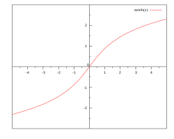
Обратный гиперболический синус

Обратный гиперболический синус (он же гиперболический синус площади) (латинское: Area sinus hyperbolicus ):

${ displaystyle operatorname {arsinh} x = ln left (x + { sqrt {x ^ {2} +1}} right)}$

Домен — это целая реальная линия .

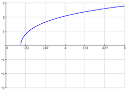
Обратный гиперболический косинус

Обратный гиперболический косинус (он же гиперболический косинус площади ) (лат. Area cosinus hyperbolicus ):

${ displaystyle operatorname {arcosh} x = ln left (x + { sqrt {x ^ {2} -1}} right)}$

Область — отрезок [1, + ∞) .

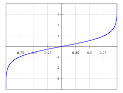
Обратный гиперболический тангенс

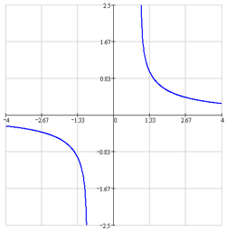
Обратный гиперболический тангенс (он же реальный гиперболический тангенс ) (лат. Area tangens hyperbolicus ):

${ displaystyle operatorname {artanh} x = { frac {1} {2}} ln left ({ frac {1 + x} {1-x}} right)}$

Область — это открытый интервал (−1, 1) .

Обратный гиперболический котангенс

Обратный гиперболический котангенс (он же гиперболический котангенс площади ) (лат. Area cotangens hyperbolicus ):

${ displaystyle operatorname {arcoth} x = { frac {1} {2}} ln left ({ frac {x + 1} {x-1}} right)}$

Область представляет собой объединение открытых интервалов (−∞, −1) и (1, + ∞) .

Обратный гиперболический секанс

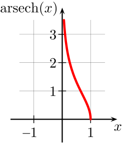
Обратный гиперболический секанс (он же гиперболический секанс площади ) (лат. Area secans hyperbolicus ):

${ displaystyle operatorname {arsech} x = ln left ({ frac {1} {x}} + { sqrt {{ frac {1} {x ^ {2}}} - 1}} right ) = ln left ({ frac {1 + { sqrt {1-x ^ {2}}}} {x}} right)}$

Область представляет собой полуоткрытый интервал (0, 1) .

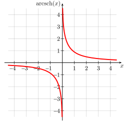
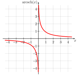
Обратный гиперболический косеканс

Обратный гиперболический косеканс (также известный как гиперболический косеканс площади ) (лат. Area cosecans hyperbolicus ):

${ displaystyle operatorname {arcsch} x = ln left ({ frac {1} {x}} + { sqrt {{ frac {1} {x ^ {2}}} + 1}} right )}$

Домен — это реальная строка с удаленным 0.

Формулы сложения

${ displaystyle operatorname {arsinh} u pm operatorname {arsinh} v = operatorname {arsinh} left (u { sqrt {1 + v ^ {2}}} pm v { sqrt {1 + u) ^ {2}}} right)}$

${ displaystyle operatorname {arcosh} u pm operatorname {arcosh} v = operatorname {arcosh} left (uv pm { sqrt {(u ^ {2} -1) (v ^ {2} -1) )}}Правильно)}$

${ displaystyle operatorname {artanh} u pm operatorname {artanh} v = operatorname {artanh} left ({ frac {u pm v} {1 pm uv}} right)}$

${ displaystyle operatorname {arcoth} u pm operatorname {arcoth} v = operatorname {arcoth} left ({ frac {1 pm uv} {u pm v}} right)}$

${ displaystyle { begin {align} operatorname {arsinh} u + operatorname {arcosh} v & = operatorname {arsinh} left (uv + { sqrt {(1 + u ^ {2}) (v ^ {2}) -1)}} right) \ & = operatorname {arcosh} left (v { sqrt {1 + u ^ {2}}} + u { sqrt {v ^ {2} -1}} вправо) end {выровнен}}}$

Другие личности

${ begin {align} 2 operatorname {arcosh} x & = operatorname {arcosh} (2x ^ {2} -1) & quad { hbox {for}} x geq 1 \ 4 operatorname {arcosh} x & = operatorname {arcosh} (8x ^ {4} -8x ^ {2} +1) & quad { hbox {for}} x geq 1 \ 2 operatorname {arsinh} x & = operatorname {arcosh } (2x ^ {2} +1) & quad { hbox {for}} x geq 0 \ 4 operatorname {arsinh} x & = operatorname {arcosh} (8x ^ {4} + 8x ^ {2 } +1) & quad { hbox {for}} x geq 0 end {выровнено}}$

${ displaystyle ln (x) = operatorname {arcosh} left ({ frac {x ^ {2} +1} {2x}} right) = operatorname {arsinh} left ({ frac {x ^ {2} -1} {2x}} right) = operatorname {artanh} left ({ frac {x ^ {2} -1} {x ^ {2} +1}} right)}$

Состав гиперболических и обратных гиперболических функций

${ displaystyle { begin {align} & sinh ( operatorname {arcosh} x) = { sqrt {x ^ {2} -1}} quad { text {for}} quad | x |> 1 \ & sinh ( operatorname {artanh} x) = { frac {x} { sqrt {1-x ^ {2}}}} quad { text {for}} quad -1 <x < 1 \ & cosh ( operatorname {arsinh} x) = { sqrt {1 + x ^ {2}}} \ & cosh ( operatorname {artanh} x) = { frac {1} { sqrt {1-x ^ {2}}}} quad { text {for}} quad -1 <x <1 \ & tanh ( operatorname {arsinh} x) = { frac {x} { sqrt {1 + x ^ {2}}}} \ & tanh ( operatorname {arcosh} x) = { frac { sqrt {x ^ {2} -1}} {x}} quad { текст {для}} quad | x |> 1 конец {выровнено}}}$

Состав обратных гиперболических и тригонометрических функций

${ displaystyle operatorname {arsinh} left ( tan alpha right) = operatorname {artanh} left ( sin alpha right) = ln left ({ frac {1+ sin alpha } { cos alpha}} right) = pm operatorname {arcosh} left ({ frac {1} { cos alpha}} right)}$

{ Displaystyle пер влево ( влево | загар альфа вправо | вправо) = - OperatorName {artanh} влево ( соз 2 альфа вправо)}

Конверсии

${ displaystyle ln x = operatorname {artanh} left ({ frac {x ^ {2} -1} {x ^ {2} +1}} right) = operatorname {arsinh} left ({ frac {x ^ {2} -1} {2x}} right) = pm operatorname {arcosh} left ({ frac {x ^ {2} +1} {2x}} right)}$

${ displaystyle operatorname {artanh} x = operatorname {arsinh} left ({ frac {x} { sqrt {1-x ^ {2}}}}} right) = pm operatorname {arcosh} left ({ frac {1} { sqrt {1-x ^ {2}}}} right)}$

${ displaystyle operatorname {arsinh} x = operatorname {artanh} left ({ frac {x} { sqrt {1 + x ^ {2}}}}} right) = pm operatorname {arcosh} влево ({ sqrt {1 + x ^ {2}}} right)}$

${ displaystyle operatorname {arcosh} x = left | operatorname {arsinh} left ({ sqrt {x ^ {2} -1}} right) right | = left | operatorname {artanh} left ({ frac { sqrt {x ^ {2} -1}} {x}} right) right |}$

Производные

${ displaystyle { begin {align} { frac {d} {dx}} operatorname {arsinh} x & {} = { frac {1} { sqrt {x ^ {2} +1}}}, { text {для всех реальных}} x \ { frac {d} {dx}} operatorname {arcosh} x & {} = { frac {1} { sqrt {x ^ {2} -1}}} , { text {для всех реальных}} x> 1 \ { frac {d} {dx}} operatorname {artanh} x & {} = { frac {1} {1-x ^ {2}}} , { text {для всех реальных}} | x | <1 \ { frac {d} {dx}} operatorname {arcoth} x & {} = { frac {1} {1-x ^ {2} }}, { text {для всех реальных}} | x |> 1 \ { frac {d} {dx}} operatorname {arsech} x & {} = { frac {-1} {x { sqrt {1-x ^ {2}}}}}, { text {для всех реальных}} x in (0,1) \ { frac {d} {dx}} operatorname {arcsch} x & {} = { frac {-1} {| x | { sqrt {1 + x ^ {2}}}}}, { text {для всех вещественных}} x { text {, кроме}} 0 \ конец {выровнен}}}$

Для примера дифференцирования: пусть θ = arsinh x , поэтому (где sinh ² θ = (sinh θ ) ² ):

${ displaystyle { frac {d , operatorname {arsinh} x} {dx}} = { frac {d theta} {d sinh theta}} = { frac {1} { cosh theta }} = { frac {1} { sqrt {1+ sinh ^ {2} theta}}} = { frac {1} { sqrt {1 + x ^ {2}}}}.}.}$

Расширения серии

Ряд расширения может быть получен для вышеуказанных функций:

${ displaystyle { begin {align} operatorname {arsinh} x & = x- left ({ frac {1} {2}} right) { frac {x ^ {3}} {3}} + left ({ frac {1 cdot 3} {2 cdot 4}} right) { frac {x ^ {5}} {5}} - left ({ frac {1 cdot 3 cdot 5 } {2 cdot 4 cdot 6}} right) { frac {x ^ {7}} {7}} pm cdots \ & = sum _ {n = 0} ^ { infty} left ({ frac {(-1) ^ {n} (2n)!} {2 ^ {2n} (n!) ^ {2}}} right) { frac {x ^ {2n + 1}} {2n + 1}}, qquad left | x right | <1 конец {выровнено}}}$

${ displaystyle { begin {align} operatorname {arcosh} x & = ln (2x) - left ( left ({ frac {1} {2}} right) { frac {x ^ {- 2 }} {2}} + left ({ frac {1 cdot 3} {2 cdot 4}} right) { frac {x ^ {- 4}} {4}} + left ({ frac {1 cdot 3 cdot 5} {2 cdot 4 cdot 6}} right) { frac {x ^ {- 6}} {6}} + cdots right) \ & = ln (2x) - sum _ {n = 1} ^ { infty} left ({ frac {(2n)!} {2 ^ {2n} (n!) ^ {2}}} right) { гидроразрыв {x ^ {- 2n}} {2n}}, qquad left | x right |> 1 end {align}}}$

${ displaystyle { begin {align} operatorname {artanh} x & = x + { frac {x ^ {3}} {3}} + { frac {x ^ {5}} {5}} + { frac {x ^ {7}} {7}} + cdots \ & = sum _ {n = 0} ^ { infty} { frac {x ^ {2n + 1}} {2n + 1}}, qquad left | x right | <1 конец {выровнено}}}$

${ displaystyle { begin {align} operatorname {arcsch} x = operatorname {arsinh} { frac {1} {x}} & = x ^ {- 1} - left ({ frac {1} { 2}} right) { frac {x ^ {- 3}} {3}} + left ({ frac {1 cdot 3} {2 cdot 4}} right) { frac {x ^ {-5}} {5}} - left ({ frac {1 cdot 3 cdot 5} {2 cdot 4 cdot 6}} right) { frac {x ^ {- 7}} { 7}} pm cdots \ & = sum _ {n = 0} ^ { infty} left ({ frac {(-1) ^ {n} (2n)!} {2 ^ {2n} (n!) ^ {2}}} right) { frac {x ^ {- (2n + 1)}} {2n + 1}}, qquad left | x right |> 1 end {выровнено }}}$

${ displaystyle { begin {align} operatorname {arsech} x = operatorname {arcosh} { frac {1} {x}} & = ln { frac {2} {x}} - left ( left ({ frac {1} {2}} right) { frac {x ^ {2}} {2}} + left ({ frac {1 cdot 3} {2 cdot 4}} справа) { frac {x ^ {4}} {4}} + left ({ frac {1 cdot 3 cdot 5} {2 cdot 4 cdot 6}} right) { frac {x ^ {6}} {6}} + cdots right) \ & = ln { frac {2} {x}} - sum _ {n = 1} ^ { infty} left ({ frac {(2n)!} {2 ^ {2n} (n!) ^ {2}}} right) { frac {x ^ {2n}} {2n}}, qquad 0 <x leq 1 конец {выровнен}}}$

${ displaystyle { begin {align} operatorname {arcoth} x = operatorname {artanh} { frac {1} {x}} & = x ^ {- 1} + { frac {x ^ {- 3} } {3}} + { frac {x ^ {- 5}} {5}} + { frac {x ^ {- 7}} {7}} + cdots \ & = sum _ {n = 0} ^ { infty} { frac {x ^ {- (2n + 1)}} {2n + 1}}, qquad left | x right |> 1 end {выровнено}}}$

Асимптотическое разложение для arsinh x дается выражением

${ displaystyle operatorname {arsinh} x = ln (2x) + sum limits _ {n = 1} ^ { infty} { left ({- 1} right) ^ {n-1} { гидроразрыв { left ({2n-1} right) !!} {2n left ({2n} right) !!}}} { frac {1} {x ^ {2n}}}}$

Основные значения в комплексной плоскости

Как функции комплексной переменной обратные гиперболические функции являются многозначными функциями, которые являются аналитическими , за исключением конечного числа точек. Для такой функции обычно определяют главное значение , которое представляет собой однозначную аналитическую функцию, которая совпадает с одной конкретной ветвью многозначной функции, в области, состоящей из комплексной плоскости, в которой конечное число дуг (обычно половина линии или сегменты ) были удалены. Эти дуги называются сечениями ветвей . Для указания ветви, то есть определения того, какое значение многозначной функции рассматривается в каждой точке, обычно определяют ее в конкретной точке и выводят значение повсюду в области определения главного значения путем аналитического продолжения . По возможности лучше определять главное значение напрямую, не обращаясь к аналитическому продолжению.

Например, для квадратного корня главное значение определяется как квадратный корень с положительной действительной частью . Это определяет однозначную аналитическую функцию, которая определена везде, за исключением неположительных действительных значений переменных (где два квадратных корня имеют нулевую действительную часть). Это главное значение функции квадратного корня обозначается ниже. Точно так же главное значение логарифма, обозначаемое ниже, определяется как значение, для которого мнимая часть имеет наименьшее абсолютное значение. Он определен везде, кроме неположительных действительных значений переменной, для которых два разных значения логарифма достигают минимума.

Для всех обратных гиперболических функций главное значение может быть определено в терминах главных значений квадратного корня и функции логарифма. Однако в некоторых случаях формулы из § Определения в терминах логарифмов не дают правильного главного значения, поскольку дают область определения, которая слишком мала и, в одном случае, не связана .

Главное значение обратного гиперболического синуса

Главное значение обратного гиперболического синуса определяется выражением

$operatorname {arsinh} z = operatorname {Log} (z + { sqrt {z ^ {2} +1}} ,) ,.$

Аргумент квадратного корня является неположительным действительным числом тогда и только тогда, когда z принадлежит одному из интервалов [ i , + i ∞) и (- i ∞, — i ] мнимой оси. Если аргумент логарифм действительный, тогда он положительный. Таким образом, эта формула определяет главное значение для arsinh с отрезками ветвей [ i , + i ∞) и (- i ∞, — i ] . Это оптимально, поскольку разрезы ветвей должны соединять особые точки i и — i на бесконечность.

Главное значение обратного гиперболического косинуса

Формула для обратного гиперболического косинуса, приведенная в § Обратный гиперболический косинус, неудобна, поскольку, как и в случае с основными значениями логарифма и квадратного корня, главное значение arcosh не может быть определено для мнимого z . Таким образом, квадратный корень необходимо разложить на множители, что приведет к

Оба главных значения квадратных корней определены, за исключением случая, когда z принадлежит действительному интервалу (−∞, 1] . Если аргумент логарифма действительный, то z действительный и имеет тот же знак. Таким образом, приведенная выше формула определяет главное значение arcosh вне действительного интервала (−∞, 1] , который, таким образом, является единственным разрезом ветви.

Основные значения обратного гиперболического тангенса и котангенса

Формулы, приведенные в § Определения в терминах логарифмов, предлагают

${ begin {align} operatorname {artanh} z & = { frac {1} {2}} operatorname {Log} left ({ frac {1 + z} {1-z}} right) \ operatorname {arcoth} z & = { frac {1} {2}} operatorname {Log} left ({ frac {z + 1} {z-1}} right) end {выровнено}}$

для определения главных значений обратного гиперболического тангенса и котангенса. В этих формулах аргумент логарифма действительный тогда и только тогда, когда z действительно. Для artanh этот аргумент находится в вещественном интервале (−∞, 0] , если z принадлежит либо (−∞, −1], либо [1, ∞) . Для arcoth аргумент логарифма находится в (−∞ , 0] , тогда и только тогда, когда z принадлежит вещественному интервалу [−1, 1] .

Следовательно, эти формулы определяют удобные главные значения, для которых сечения ветвей равны (−∞, −1] и [1, ∞) для обратного гиперболического тангенса и [−1, 1] для обратного гиперболического котангенса.

Ввиду лучшей численной оценки вблизи сечений ветвей некоторые авторы используют следующие определения главных значений, хотя второе вводит устранимую особенность при z = 0 . Два определения различаются для реальных значений с . Для реальных значений с различаются .

${ displaystyle { begin {align} operatorname {artanh} z & = { tfrac {1} {2}} operatorname {Log} left ({1 + z} right) - { tfrac {1} { 2}} operatorname {Log} left ({1-z} right) \ operatorname {arcoth} z & = { tfrac {1} {2}} operatorname {Log} left ({1+ { frac {1} {z}}} right) - { tfrac {1} {2}} operatorname {Log} left ({1 - { frac {1} {z}}} right) конец {выровнен}}}$

Главное значение обратного гиперболического косеканса

Для обратного гиперболического косеканса главное значение определяется как

$operatorname {arcsch} z = operatorname {Log} left ({ frac {1} {z}} + { sqrt {{ frac {1} {z ^ {2}}} + 1}} , Правильно)$

Он определяется, когда аргументы логарифма и квадратного корня не являются неположительными действительными числами. Таким образом, главное значение квадратного корня определяется за пределами интервала [- i , i ] мнимой прямой. Если аргумент логарифма действительный, тогда z — ненулевое действительное число, и это означает, что аргумент логарифма положительный.

Таким образом, главное значение определяется по приведенной выше формуле вне отрезка ветви , состоящего из интервала [- i , i ] воображаемой прямой.

При z = 0 есть особая точка, которая входит в разрез ветви.

Главное значение обратного гиперболического секанса

Здесь, как и в случае обратного гиперболического косинуса, мы должны факторизовать квадратный корень. Это дает главное значение

${ displaystyle operatorname {arsech} z = operatorname {Log} left ({ frac {1} {z}} + { sqrt {{ frac {1} {z}} + 1}} , { sqrt {{ frac {1} {z}} - 1}} right).}$

Если аргумент квадратного корня вещественный, то z вещественно, и отсюда следует, что определены оба главных значения квадратных корней, за исключением случая, когда z вещественно и принадлежит одному из интервалов (−∞, 0] и [1, + ∞) . Если аргумент логарифма действительный и отрицательный, то z также действительный и отрицательный. Отсюда следует, что главное значение arsech корректно определяется указанной выше формулой вне двух разрезов ветвей , вещественных интервалов (−∞, 0] и [1, + ∞) .

При z = 0 имеется особая точка, входящая в одно из сечений ветвления.

Графическое представление

В следующем графическом представлении главных значений обратных гиперболических функций сечения ветвей выглядят как разрывы цвета. Тот факт, что все сечения ветвей выглядят как разрывы, показывает, что эти главные значения не могут быть расширены до аналитических функций, определенных для более крупных областей. Другими словами, определенные выше сечения ветвей минимальны.

Смотрите также

Комплексный логарифм
Распределение гиперболического секанса
ISO 80000-2
Список интегралов обратных гиперболических функций

использованная литература

Библиография

Герберт Буземанн и Пол Дж. Келли (1953) Проективная геометрия и проективные метрики , стр. 207, Academic Press .

внешние ссылки

«Обратные гиперболические функции» , Энциклопедия математики , EMS Press , 2001 [1994]

Источник

Notation[edit]

Definitions in terms of logarithms[edit]

Addition formulae[edit]

Other identities[edit]

Composition of hyperbolic and inverse hyperbolic functions[edit]

Composition of inverse hyperbolic and circular functions[edit]

Conversions[edit]

Derivatives[edit]

Series expansions[edit]

Principal values in the complex plane[edit]

Principal value of the inverse hyperbolic sine[edit]

Principal value of the inverse hyperbolic cosine[edit]

Principal values of the inverse hyperbolic tangent and cotangent[edit]

Principal value of the inverse hyperbolic cosecant[edit]

Principal value of the inverse hyperbolic secant[edit]

Graphical representation[edit]

See also[edit]

References[edit]

Bibliography[edit]

External links[edit]

Определения функций

Разложение в ряд

Производные

Комбинация гиперболических и обратных гиперболических функций

Дополнительные формулы

См. также

Источники

Ссылки

Содержание

Определения функций

Разложение в ряд

Производные

Комбинация гиперболических и обратных гиперболических функций

Дополнительные формулы

См. также

Источники

Ссылки

Обозначение

Определения в терминах логарифмов

Обратный гиперболический синус

Обратный гиперболический косинус

Обратный гиперболический тангенс

Обратный гиперболический котангенс

Обратный гиперболический секанс

Обратный гиперболический косеканс

Формулы сложения

Другие личности

Состав гиперболических и обратных гиперболических функций

Состав обратных гиперболических и тригонометрических функций

Конверсии

Производные

Расширения серии

Основные значения в комплексной плоскости

Главное значение обратного гиперболического синуса

Главное значение обратного гиперболического косинуса

Основные значения обратного гиперболического тангенса и котангенса

Главное значение обратного гиперболического косеканса

Главное значение обратного гиперболического секанса

Графическое представление

Смотрите также

использованная литература

Библиография

внешние ссылки

Не пропустите также: